The downloaded file - "Shift detection.xla" - is an Excel add-in. It can be placed in any folder of your choice and can be run from there. For more convenience, you can add it to the existing list of add-ins. In Excel, go to Tools --> Add-Ins... to open a list of existing add-ins. Click Browse to navigate to the folder where you saved "Shift detection.xla." Choose the file and click OK. Now, when you have "Shift detection" in the list, you can check (uncheck) the associated box to enable (disable) it. To remove it permanently, uncheck the box and delete the file "Shift detection.xla" from its original folder. When you go Tools --> Add-Ins and click Browse, you will receive the message "Cannot find add-in [path]/Shift detection.xla. Delete from list?" Click Yes to finish. After the installation you should see the Shifts menu at the end of the main worksheet menu bar as in Fig. 1 below.

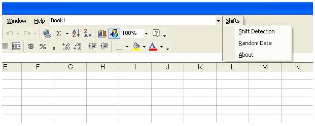
Fig. 1. The Shifts menu after the installation.

Open a new workbook or the one that contains your data. The time series are organized by columns. The first column is always the time of observations, e.g., years. The first row must always contain labels (names of time series). These labels will be used to name new output worksheets. The time series in the data matrix can start and end at different years, but no missing data within an individual time series is allowed.

If you want to experiment with normally distributed random numbers, click Shifts --> Random Data to populate the spreadsheet. Maximum number of time series is 250.

Click Shifts --> Shift Detection to open the entry form as in Fig. 2. The entire data range is automatically selected. You can select your own data range by clicking the button with underscore.

There are two parameters that control the magnitude and scale of the regimes to be detected. The significance level is the level at which the null hypothesis that the mean values of the two regimes are equal is rejected by the two-tailed Student t-test. The lower the significance level, the larger the magnitude of the shift should be in order to be detected. It is important to note that if the regime shift is detected, the difference between the mean values of the old and new regimes is statistically significant at least at the given level. The program also calculates the actual significance level between the two regimes.

The cut-off length is similar to the 100% cut-off point in filtering. The regimes that are longer than the cut-off length will all be detected. If the regimes are shorter than the cut-off length, the probability for them to be detected reduces proportionally to their length. Some of them, however, may still be selected if the magnitude of the shift is significant enough. Generally speaking, the shorter the cut-off length, the shorter the regimes that will be selected (and vice versa), but it's not always true. The reason is that the cut-off length also affects the critical magnitude of the shift between the regimes to be detected. For example, the difference of two units between the mean values of two regimes is statistically significant at the 0.01 level if the cut-off length is 10 years. But if the cut-off length is reduced to 5 years, the critical magnitude of the shift increases (for the same significance level), and the regimes may not be selected. It is recommended to experiment first with different significance levels and cut-off lengths to better understand their mutual effect on regime detection.

The program also requires the Huber's weight parameter that controls the weights assigned to the outliers (see below for more information). Therefore this parameter affects the average value of the regimes .

For each time series, the program calculates the regime shift index (RSI), the mean value of the regimes with equal and unequal weights, regime length, final confidence levels for the shifts and the weights of the outliers. This information for each variable is placed in a separate worksheet along with the corresponding graphs. The program also calculates the combined RSI ("Summary" worksheet) and residuals after the stepwise regime function is removed ("Residuals" worksheet). You can apply the method again to the residual worksheet, if you wish, but it has to be renamed first if the output is placed in the same workbook. The residuals can also be used to check for regime shift in the variance (no need to rename the worksheet in this case).

Due to outliers, the average is not representative for the mean value of the regimes, and this may significantly affect the results of the regime shift detection. Ideally the weight for the data value should be chosen such that it is small if that value is considered as an outlier. To handle the outliers, the program uses the Huber's weight function, which is calculated here as

where anomaly is the deviation from the expected mean value of the new regime normalized by the standard deviation averaged for all consecutive sections of the cut-off length in the series. If anomalies are less than or equal to the value of the parameter then their weights are equal to one. Otherwise, the weights are inversely proportional to the distance from the expected mean value of the new regime.

After the timing of the regime shifts is determined, the mean values of the regimes are determined using the following iterative procedure. First, a simple unweihed arithmetic mean is calculated as the initial estimate of the mean value of the regime. Then a weighed mean is calculated with the weights determined by the distance from that first estimate. The procedure is repeated one more time with the new estimate of the regime mean.

Figure 3 below illustrates the effect of the outliers on the timing of regime shifts in mean winter (DJF) temperature in central England for the period 1900-1933. The top graph shows that if the Huber's weight parameter is set to 6 (i.e., all temperature values that are less than six standard deviations have equal weights), a regime shift is detected 1920. The temperature value for 1917, however, appears to be an outlier. Reducing the Huber's weight parameter to 1 (bottom graph) changes the regime shift year to 1911.

Fig. 3. The results of the regime shift detection for the winter (DJF) surface air temperature in central England using two different Huber's weight parameters: 6 (top panel) and 1 (bottom panel). Note changes in the onset and termination of the second regime.

It is assumed that all regime shifts in the mean are removed, that is, the values of the time series are deviations from the zero mean. The same two parameters, the significance level and the cut-off length, control the magnitude of the shifts and the length of the regimes to be detected. The Huber's weight function is not used for the variance.

12/03/2004: Ver. 1 released.

06/07/2005: Ver. 2 released. The Huber's weight function is added to handle the outliers.